the Creative Commons Attribution 4.0 License.
the Creative Commons Attribution 4.0 License.
 | 21 Feb 2020
Sampling fossil floras for the study of insect herbivory: how many leaves is enough?
S. Augusta Maccracken
Conrad C. Labandeira
Despite the great importance of plant–insect interactions to the functioning of terrestrial ecosystems, many temporal gaps exist in our knowledge of insect herbivory in deep time. Subsampling of fossil leaves, and subsequent extrapolation of results to the entire flora from which they came, is practiced inconsistently and according to inconsistent, often arbitrary criteria. Here we compare herbivory data from three exhaustively sampled fossil floras to establish guidelines for subsampling in future studies. The impact of various subsampling routines is evaluated for three of the most common metrics of insect herbivory: damage type diversity, nonmetric multidimensional scaling, and the herbivory index. The findings presented here suggest that a minimum fragment size threshold of 1 cm2 always yields accurate results and that a higher threshold of 2 cm2 should yield accurate results for plant hosts that are not polyphyletic form taxa. Due to the structural variability of the plant hosts examined here, no other a priori subsampling strategy yields consistently accurate results. The best approach may be a sequential sampling routine in which sampling continues until the 100 most recently sampled leaves have caused no change to the mean value or confidence interval for damage type diversity and have caused minimal or no change to the herbivory index. For nonmetric multidimensional scaling, at least 1000 cm2 of leaf surface area should be examined and prediction intervals should be generated to verify the relative positions of all points. Future studies should evaluate the impact of subsampling routines on floras that are collected based on different criteria, such as angiosperm floras for which the only specimens collected are those that are at least 50 % complete.
- Article
(5465 KB) -
Supplement
(16984 KB) - BibTeX
- EndNote


Plants serve as the foundation of many terrestrial ecosystems, and insects have herbivorized plants for hundreds of millions of years (Labandeira et al., 2013). The fossil record provides data on plant–insect interactions that encompass far longer time spans than can be examined in laboratory studies, yielding insight into such timely issues as the response of insect herbivores to climate change (Currano et al., 2010). Fossil evidence of insect herbivory includes coprolites (Slater et al., 2012) and traces of insect feeding on roots (Strullu-Derrien et al., 2012), wood (Pires and Sommer, 2009), seeds (Schachat et al., 2014, 2015), fruit (Meng et al., 2017), and leaves (Pinheiro et al., 2016), with leaves being the most intensely studied. Insect herbivory on leaves and other plant organs has been categorized qualitatively using the “damage type” (DT) system (Labandeira et al., 2007).
Studies of insect herbivory in the fossil record vary tremendously in their intensity of coverage. At one extreme is the description of a single, notable DT on a single plant taxon (Béthoux et al., 2004; Iannuzzi and Labandeira, 2008), which may occur on a single specimen (Jud and Sohn, 2016); at the other extreme is the documentation of all DTs on all taxa in an entire fossil flora, which can contain thousands or even tens of thousands of specimens (Labandeira et al., 2018). Many authors have taken intermediate approaches, for example, by documenting all DTs on a subset of leaves from various taxa (Filho et al., 2019), by documenting DTs for a specific behavior such as galling (Knor et al., 2013), or by categorizing feeding damage at a coarser scale than the DT system, such as the level of functional feeding group (Smith, 2008; McLoughlin et al., 2015). Some studies are based on exhaustive examinations of a single plant lineage at multiple fossil assemblages (Ding et al., 2015; Glasspool et al., 2003; Kodrul et al., 2018) on the premise that controlling for plant-host affinity will produce more robust conclusions regarding the evolution of plant–insect interactions. However, because extant species, genera, and families do not have fossil records that extend back to the Paleozoic, data from entire assemblages must be used to compare herbivory on longer timescales.
Such data remain scant. A recent meta-analysis included DT data from 50 exhaustively sampled floras (Pinheiro et al., 2016). These 50 floras amount to an average of 1 flora per 7.7 million years for all habitats across the planet. Many of these floras are separated by long temporal gaps: one of these gaps in the above study approaches 100 million years in length and another exceeds 165 million years. The Carboniferous and Jurassic periods are not represented by any such floras, and the Triassic and Cretaceous periods are represented by only two floras each. The meta-analysis examined DT diversity only and included many studies for which quantitative data (measurements of herbivorized leaf area) are not available. This study raises two main issues regarding current knowledge about the documentation of arthropod herbivory across time. First, there is an absence of available quantitative data that severely limits the conclusions that can be drawn from existing studies. Second, far more studies are needed across all intervals to document patterns of insect herbivory, as discussed by the authors (Pinheiro et al., 2016). The rate at which fossil floras are examined for insect herbivory appears to be increasing, as demonstrated by the 15 recent studies that were not included in the above meta-analysis (see Supplement), presumably because they were published after the analysis was conducted.
The field of ancient plant–insect associations is rife with possibilities for understanding the fossil record of arthropod herbivory because of ample paleobotanical collections of museums, universities, and other research institutions across the world. Although fossil plant collections of such institutions vary immensely in size, collection techniques, scope, level of plant identification, and preservation, these collections permit analyses for insect damage. However, the major impediments to the study of large paleobotanical collections are time and research funding. Visits to collections that are of sufficient length to allow collection of quantitative data for thousands of leaves are often cost-prohibitive. It is, therefore, imperative to discern whether and how the data from a subset of specimens could be used to extrapolate patterns of insect herbivory for all specimens pertaining to a given plant host or assemblage. Furthermore, it would be useful to know whether the common collecting technique of discarding small leaf fragments, such as those below 1 cm2 in surface area, distorts the overall trends in insect herbivory for a particular flora. Subsampling of additional paleobotanical collections is key to addressing these issues.
1.1 Subsampling of ecological data
Subsampling can be conducted in one of two ways. Subsampling can occur after data collection with the aim of standardizing sampling procedures (Droissert et al., 2012) or can occur before data collection, with the aims of standardizing sampling procedures and reducing collection effort (Bowen and Freeman, 1998). Subsampling is standard practice among neontologists; for example, transects and quadrats are very commonly used to subsample extant populations and communities (Pilliod and Arkle, 2013).
When fossil floras are studied for insect herbivory, they are typically examined exhaustively: all leaves above a certain size threshold, or all leaves that are at least 50 % complete, are sampled. Subsampling strategies, analogous to the transects and quadrats used by neontologists, could be applied to insect herbivory in the fossil record. Such an approach would result in a reduction in the effort required to examine a single flora and would increase the rate at which such floras could be studied. However, at present, no guidelines are available to ensure consistent subsampling of fossil leaves or to ensure that subsampling routines adequately capture the trends that emerge from complete datasets. The aims of the present contribution are to test the effects of various subsampling routines on herbivorized fossil leaves and to establish guidelines for subsampling in future studies.
1.2 Metrics of insect herbivory
In previous contributions, four metrics have typically been used to compare insect herbivory across fossil host plants and assemblages. These metrics address three aspects of plant–insect interactions.
Damage type diversity (DT diversity) addresses the diversity of damage types for an individual plant host or assemblage. DT diversity is typically reported either unstandardized (Pinheiro et al., 2016) or standardized with sample-based rarefaction in which each plant specimen is treated as a sample (Currano et al., 2011; Wappler and Denk, 2011). We recommend standardization with rarefaction curves that are scaled by the amount of leaf surface area examined (Schachat et al., 2018).
Nonmetric multidimensional scaling (NMDS) is an unconstrained ordination method (Kruskal and Wish, 1978) applied to address differences in herbivory across different plant hosts and assemblages. Plant hosts with identical levels of DT diversity (e.g., 5 DTs each) could have an identical suite of DTs (e.g., DTs 1, 2, 3, 4, and 5) or completely different suites of DTs (e.g., DTs 1, 2, 3, 4, and 5 at one site and DTs 6, 7, 8, 9, and 10 at the other site). NMDS addresses these potential differences in DT community composition. NMDS is typically performed with data at the level of functional feeding group rather than at the DT level (Wappler et al., 2009; Currano et al., 2010; Xu et al., 2018); functional feeding groups are the broad categories, such as galling and leaf mining, to which each DT is assigned. The use of coarser functional-feeding-group data is often intended to increase the signal-to-noise ratio (Currano et al., 2010).
The herbivory index (HI) is the percentage of leaf surface area removed by herbivores. The HI measures the intensity of insect herbivory, unlike DT diversity and NMDS, which reflect different aspects of the diversity of herbivory. Plant hosts with the same suite of DTs will be indistinguishable in terms of DT diversity and NMDS but will yield different herbivory indices if they vary in the amount of surface area removed by herbivores.
The last metric is the proportion of plant specimens showing evidence of insect damage. We consider use of this metric to be inadvisable for the following reasons. First, if all specimens are examined regardless of whether they are at least 50 % complete – a necessary approach for certain plant hosts such as Taeniopteris Brongniart from the early Permian of Texas – this metric may be biased if the degree of fragmentation varies by plant host or assemblage. Second, this metric may be biased if average leaf size varies by plant host or assemblage. Third, this metric and the HI are both intended to measure the same thing – the intensity of insect herbivory – and the HI is not biased by fragmentation or leaf size. Consequently, this renders moot the use of the proportion of plant specimens exhibiting insect damage.
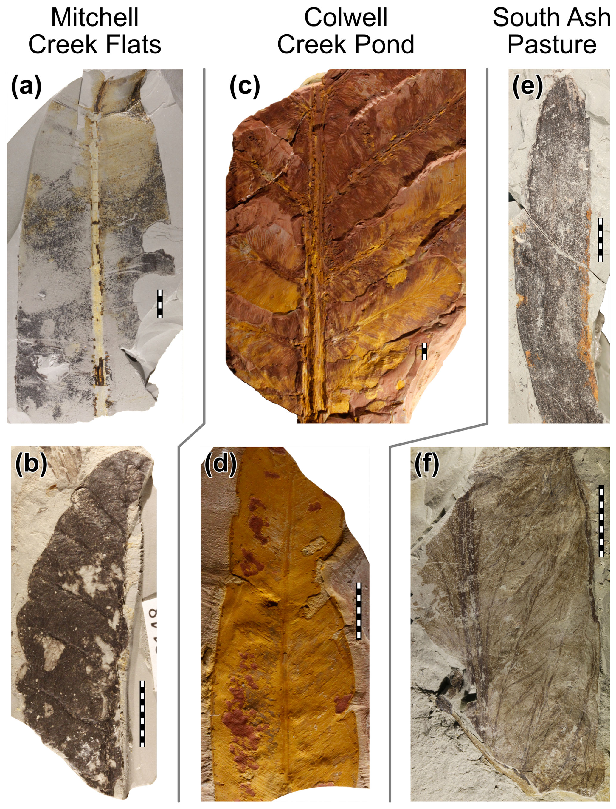
Figure 1Exemplars of the plant hosts analyzed in this study. (a) Taeniopteris from Mitchell Creek Flats, specimen USNM-612206. (b) Zeilleropteris from Mitchell Creek Flats, specimen USNM-612216. (c) Auritifolia waggoneri from Colwell Creek Pond, specimen USNM-559854. (d) Taeniopteris from Colwell Creek Pond, specimen USNM-559818. (e) Johniphyllum multinerve from South Ash Pasture, specimen USNM-520377. (f) Euparyphoselis gibsonii from South Ash Pasture, specimen USNM-520383.
1.3 The Permian of Texas
The data used here are from three Permian fossil assemblages from north-central Texas that are dominated by broadleaf plant hosts (Fig. 1). These assemblages predate the origin of angiosperms (Brenner, 1996) and the majority of plant hosts discussed here are gymnosperms. The oldest assemblage, from Mitchell Creek Flats (MCF), is dated as early Permian (Chaney et al., 2005). The form genus Taeniopteris is the primarily dominant plant host at MCF but is represented by only 104 specimens, whereas the gigantopterid seed plant Zeilleropteris Mamay sp. is the secondarily dominant plant host (Schachat et al., 2015). The assemblage from Colwell Creek Pond (CCP) is slightly younger than that from MCF and contains the primarily dominant plant hosts Auritifolia waggoneri Chaney, Mamay, DiMichele and Kerp, a peltasperm, and Taeniopteris, the form genus. Each are represented by over 400 specimens (Schachat et al., 2014). The secondarily dominant plant host at CCP is Evolsonia texana Mamay, a gigantopterid, as at MCF. The third assemblage, from the middle Permian, derives from South Ash Pasture (SAP) (Maccracken and Labandeira, 2019; Looy and Duijnstee, 2019). The primarily dominant plant host at SAP is the broadleaf conifer Johniphyllum multinerve Looy and Duijnstee, represented by over 400 specimens. The secondarily dominant plant host is, as at MCF and CCP, a gigantopterid: Euparyphoselis gibsonii DiMichele, Looy and Chaney. At all three sites, all specimens over 0.5 cm2 in surface area were analyzed for insect herbivory. Two other assemblages from the Permian of Texas, at the Coprolite Bone Bed and Taint localities, have also been analyzed for herbivory (Beck and Labandeira, 1998; Labandeira and Allen, 2007), as has one assemblage from the uppermost Carboniferous of Texas (Xu et al., 2018), but the original data are only available for MCF, CCP, and SAP.
Three plant hosts are represented by over 400 specimens: the codominant Auritifolia waggoneri and Taeniopteris spp. at CCP and Johniphyllum multinerve at SAP. However, the dominant plant at MCF is Taeniopteris spp., consisting of slightly more than 100 specimens. These contrasting abundance profiles illustrate the variability of sample sizes within fossil floras. A. waggoneri is a possible comioid seed plant (Chaney et al., 2009) that has compound leaves and is represented at CCP by specimens that range from large, complete fronds to minute fragments. All material identifiable as A. waggoneri was measured for insect herbivory. This material includes pinnae together with any attached petioles and axes, with pinnae accounting for the vast majority of surface area measured for this plant host. By contrast, Taeniopteris is a form taxon that is certainly polyphyletic at CCP: the majority of these specimens are interpreted to be of cycadophyte affinities and thus gymnospermous, but some specimens show evidence of probable spore-bearing fructifications and, therefore, cannot be assigned to any seed plant lineage. It is for this reason that the designation, Taeniopteris spp., is given, to denote that this leaf type contains two or more distantly related but indistinguishable plant taxa. Due to the elongate leaf shape and variable size of Taeniopteris, it is impossible to determine whether a given fragment represents more or less than 50 % of the original leaf. Unlike Auritifolia waggoneri, Taeniopteris spp. is not known to be represented by any affiliated axes preserved at CCP.
Johniphyllum multinerve at SAP is variable in morphology; when SAP was initially examined for insect herbivory, the broadleaf conifer specimens were divided into two distinct morphotypes based on leaf width and vein thickness. These two morphotypes were later assigned to the same species (Looy and Duijnstee, 2019). Plasticity and structural variability of leaf morphology are common throughout the plant kingdom, and multiple leaf forms are frequently found on the same individual. Plasticity may be the result of environmental factors such as sunlight (Sarijeva et al., 2007), biological interactions such as induced plant-host defenses from attacking insect herbivores (Karban and Baldwin, 2007), leaf age (England and Attiwill, 2006), or reproductive variability such as the fertile and sterile foliage of ferns (Gifford and Foster, 1989). In turn, this plasticity may impact the extent of insect-mediated herbivory on different leaf forms. The amount of insect damage was considerably higher on one form than on the other, and the separation of these forms allows quantification of the potential differences in herbivory between forms belonging to the same nominal species. Because J. multinerve at SAP can be confidently divided into two discrete forms, this plant host can be considered to be even more morphologically variable than Taeniopteris spp. of CCP, despite being a monophyletic taxon.
All analyses were conducted in R, version 3.4.2 (R Development Core Team, 2017), and all figures were produced with the package ggplot2, version 2.2.1 (Wickham, 2009).
2.1 Damage type diversity and the herbivory index
Damage type diversity (DT diversity) and the herbivory index (HI), or percentage of leaf area removed, were analyzed under various subsampling routines. Ninety-five percent confidence intervals were calculated for all analyses of these two metrics. Confidence intervals were initially calculated for the complete dataset for each plant host; no subsampling routines were performed. All confidence intervals were calculated using 100 000 bootstrap replicates.
The subsampling routines fall into four categories. The first subsampling category is random: 100 and 200 specimens were randomly sampled for each plant host. The second subsampling category is size: the 100 and 200 specimens with the highest surface area were sampled. To represent a more realistic approach, another subsampling routine was conducted in which 200 of the largest 250 specimens were sampled. This process was carried out because it may be impossible to precisely identify the largest 200 specimens without first digitizing and measuring their surface area, a time-consuming process. The third category of subsampling routines uses a minimum size cutoff: the only specimens sampled were those above 1, 2, or 5 cm2 in total surface area. For Taeniopteris spp. at MCF and for all secondarily dominant, gigantopterid plant hosts, only the third category of subsampling routines was performed because an insufficient number of specimens was available for the first two categories of subsampling routines.
The last subsampling routine is by size but uses a sequential approach to provide a more detailed view of how mean values and confidence intervals respond to increases in sample size. First, the 100 largest specimens per plant host were sampled as above. Then the next 10 largest specimens – the 101st- through 110th-largest specimens – were added to the sample. This was then followed by the next 10 largest specimens, and the process continued until all specimens had been sampled. This subsampling routine can only be performed for plant hosts represented by at least 110 specimens.
2.2 Nonmetric multidimensional scaling
To address the impact of subsampling on the differentiation of herbivore communities, we performed ordinations of functional-feeding-group (FFG) data at different levels of sampling. Fungal damage was excluded from all NMDS analyses. All NMDS analyses were conducted with the R package vegan, version 2.4–4 (Oksanen et al., 2018).
2.2.1 Data used for NMDS
In light of the importance of surface area to analyses of insect herbivory (Schachat et al., 2018), the ideal data used for NMDS would be the amount of leaf surface area damaged by insect herbivores corresponding to each FFG. However, such data are not available for the assemblages in question or for any fossil assemblages that we are aware of. The data collected for CCP, SAP, and MCF include the total amount of leaf area damaged by herbivores for each specimen, but these surface-area measurements are not partitioned by DT or by FFG. Therefore, for specimens with multiple FFGs, the amount of surface area corresponding to each FFG is unknown.
We performed NMDS using four types of data. First, we tallied the number of specimens sampled on which each FFG was observed. This method allows for the inclusion of all specimens in the original datasets but is susceptible to biases introduced by the varying degrees of fragmentation at the different assemblages. Second, we omitted all specimens on which multiple FFGs were observed, and then we summed the amount of leaf area corresponding to damage in each FFG. This method is robust to biases introduced by the varying degrees of fragmentation at the different assemblages but necessitates the exclusion of 268 specimens. However, because the vast majority (256 of 268, or 95.52 %) of the excluded specimens are from CCP, the site represented by the highest amount of surface area, the exclusion of these specimens had a negligible impact on the thresholds at which specimens could be subsampled for all three assemblages. Third, we again used surface-area data but combined hole feeding, margin feeding, and surface feeding – the three types of external foliage feeding seen at CCP, MCF, and SAP – into a single external foliage feeding “super FFG”. The combination of these FFGs reduced the number of specimens excluded from the dataset from 268 to 262 and can be justified ecologically on the grounds that these three FFGs all require mandibulate mouthparts. Although margin feeding, hole feeding, skeletonization, and surface feeding of external foliage feeders generally are considered four separate FFGs, the modifications of mouthpart structure that are used for detecting, accessing, and processing foliar tissue are minor when compared to other mouthpart types. The planar and chiseled mandibles for delaminating surface tissue layers in surface feeding, or the sharp, incisiform mandibles and maxillary elements for puncturing through the entire leaf in hole feeding, are subtle distinctions compared to the stylate ensembles of piercer and suckers or the projecting, dorsoventrally flattened mouthparts of leaf miners (Labandeira, 1997).
For the fourth type of data, we tallied the number of specimens sampled on which each FFG was observed, but we discarded data from Johniphyllum multinerve at SAP and from Auritifolia waggoneri at CCP following the guidelines established below. Because the mean and confidence interval for DT diversity did not change for J. multinerve between the 240th- and 340th-largest specimens, and because we recommend sampling until the most recent 100 specimens sampled do not change the mean or confidence interval for DT diversity, we discarded the 341st-largest through the smallest specimens – all specimens with a surface area below 1.306 cm2 – from this species. Similarly, because the mean and confidence interval for DT diversity did not change for A. waggoneri between the 220th- and 320th-largest specimens, we discarded the 321st-largest through the smallest specimens – all specimens with a surface area below 3.7 cm2 – from this species.
2.2.2 Computation of NMDS
Because our NMDS analyses incorporate two types of random data – the specimens sampled in each subsampling routine and the point at which the NMDS analysis is initialized – each analysis was repeated nine times, setting the seed in R with the set.seed() function and varying the seed from 1 to 9. Fungal damage, which was noted on leaves at CCP (Schachat et al., 2014), was omitted from these analyses due to its limited relevance to insect herbivore communities.
Entire assemblages were subsampled at 250, 500, 750, 1000, and 1250 cm2 of leaf surface area, and primarily dominant plant hosts were subsampled at 250, 500, 750, and 1000 cm2 of leaf surface area. For each NMDS plot, data from each assemblage/plant host were subsampled 500 times.
A Bray–Curtis distance matrix was computed for each subsampled dataset and used for the NMDS ordinations. All plots are presented as supplemental data. In each plot, all 500 points per plant host/assemblage are presented, together with ellipses representing the 84 % prediction interval for the location of each centroid, produced with the stat_ellipse function in ggplot2.
2.2.3 Interpretation of NMDS
We addressed two fundamentally different questions pertaining to NMDS. The first question is whether the relative positions of the centroids of subsampled data accurately reflect their relative positions if calculated from complete datasets. If two 84 % prediction intervals do not overlap then we assume, with a Type I error rate below 0.05 (Gotelli and Colwell, 2011), that the leaf area sampled is sufficient to capture the true relative positions of the assemblages/plant hosts in question.
The second question is whether two assemblages/plant hosts are significantly different from each other in the context of NMDS. To answer this question we evaluated the null hypothesis that the distances between centroids were indistinguishable from the distances between centroids of the same assemblage/plant host sampled twice. We sampled the most variable plant host (Johniphyllum multinerve at SAP) and the most variable assemblage (SAP) 1000 times, ran NMDS, randomly divided the points into two sets of 500 each, and calculated the distance between the centroids of the two sets of points. This procedure was repeated 1000 times for each amount of surface area. For each pair of assemblages/plant hosts evaluated, the p value for the distinctiveness of their herbivore communities was calculated as the proportion of tests of the null hypothesis in which the distance between the two simulated centroids is less than the distance between the true centroids being tested.
The 84 % prediction intervals are far wider than confidence intervals would be. For this reason, two assemblages/plant hosts whose prediction intervals do not overlap will have significantly different herbivore communities as evaluated by the hypothesis test discussed above. However, two assemblages/plant hosts whose prediction intervals do overlap may or may not have significantly different herbivore communities. The use of prediction intervals would, therefore, be overly conservative for the designation of significantly different herbivore communities.
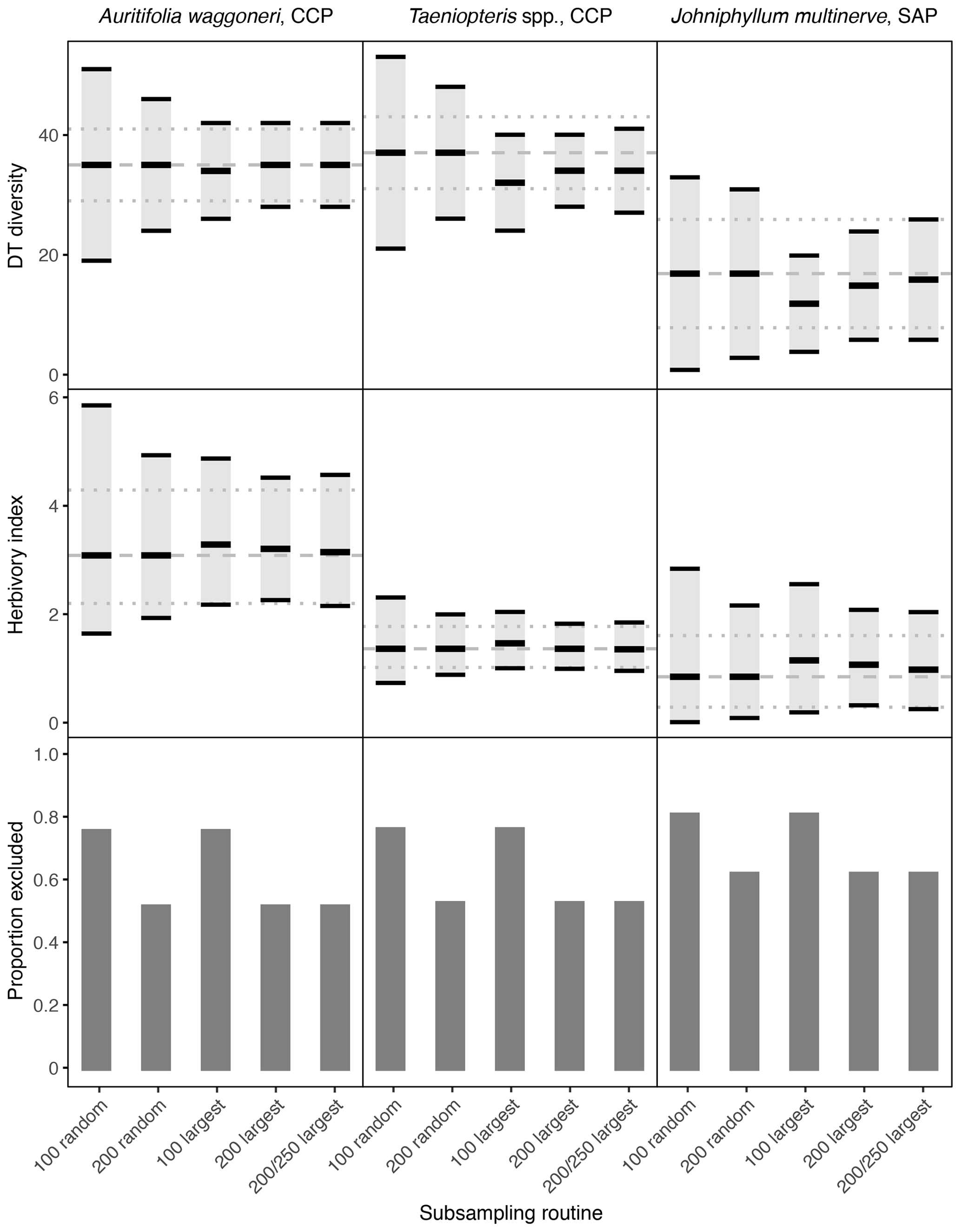
Figure 2Damage type (DT) diversity, the herbivory index (percentage of leaf area removed), and the proportion of specimens excluded, calculated with different subsampling routines for the three primarily dominant Permian plant hosts represented by 400 or more specimens. The dashed gray line represents the mean value calculated from the complete datasets, and the dotted gray lines represent the 95 % confidence intervals calculated from the complete datasets. For the complete datasets, all specimens with a surface area above 0.5 cm2 were examined. The 95 % confidence interval for each subsampling routine is represented by a light gray rectangle bounded by black lines. The thick black lines represent the mean values for each subsampling routine.
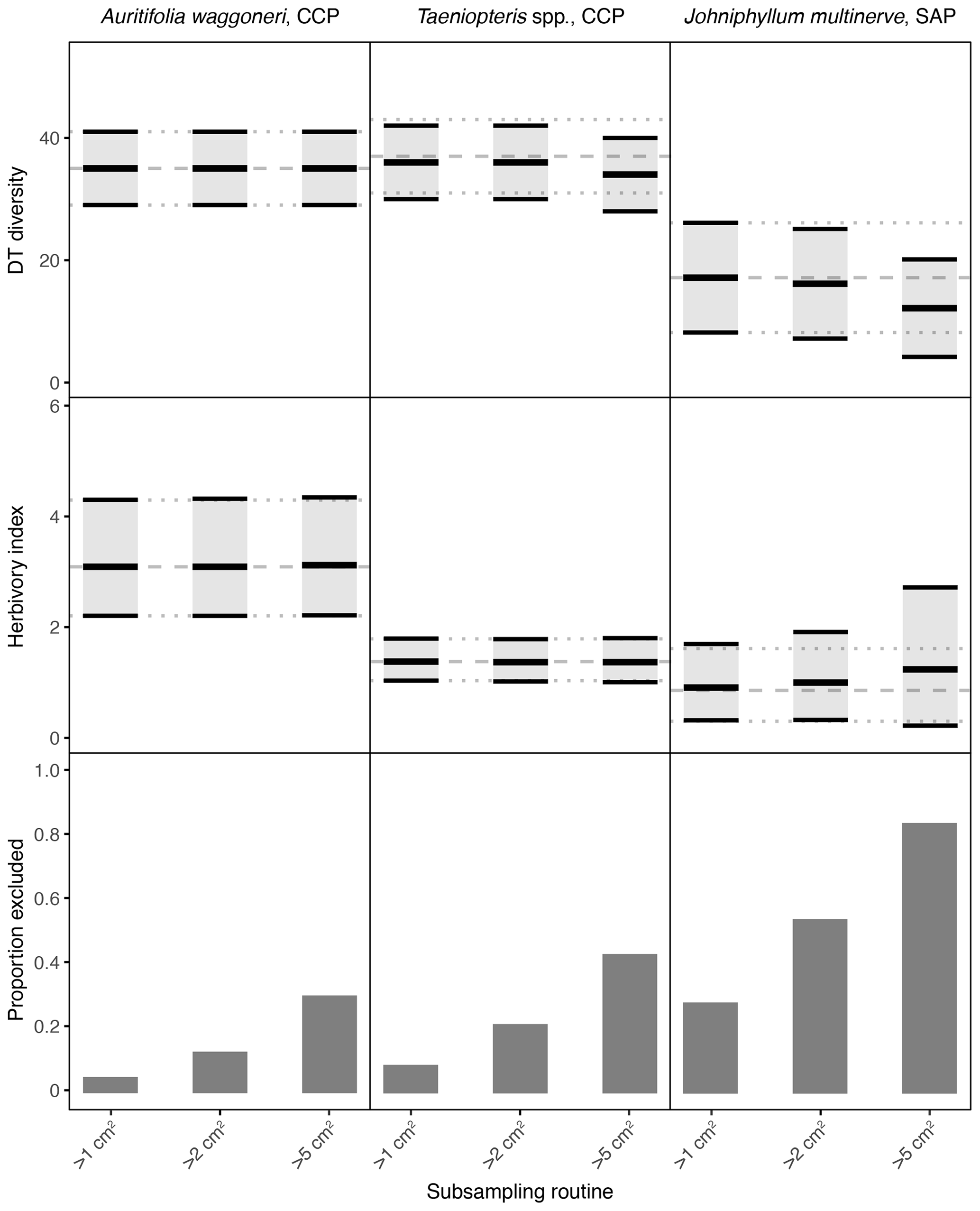
Figure 3Damage type (DT) diversity, the herbivory index (percentage of leaf area removed), and the proportion of specimens excluded, calculated with different specimen area restrictions, for the three primarily dominant Permian plant hosts represented by 400 or more specimens. The dashed gray line represents the mean value calculated for the complete dataset, and the dotted gray lines represent the 95 % confidence intervals for the complete dataset. For the complete datasets, all specimens with a surface area above 0.5 cm2 were examined. The 95 % confidence interval for each subsampling routine is represented by a light gray rectangle bounded by black lines. The thick black lines represent the mean values for each subsampling routine.
3.1 Sampling of complete datasets
Among the primarily dominant plant hosts at CCP and SAP, represented by 400 or more specimens, the complete datasets yield nonoverlapping confidence intervals for each plant host (Figs. 2, 3). Auritifolia waggoneri and Taeniopteris spp. at CCP have similar DT diversity, which is higher than the DT diversity of Johniphyllum multinerve at SAP. A. waggoneri has a higher herbivory index than either Taeniopteris spp. at CCP or J. multinerve at SAP.
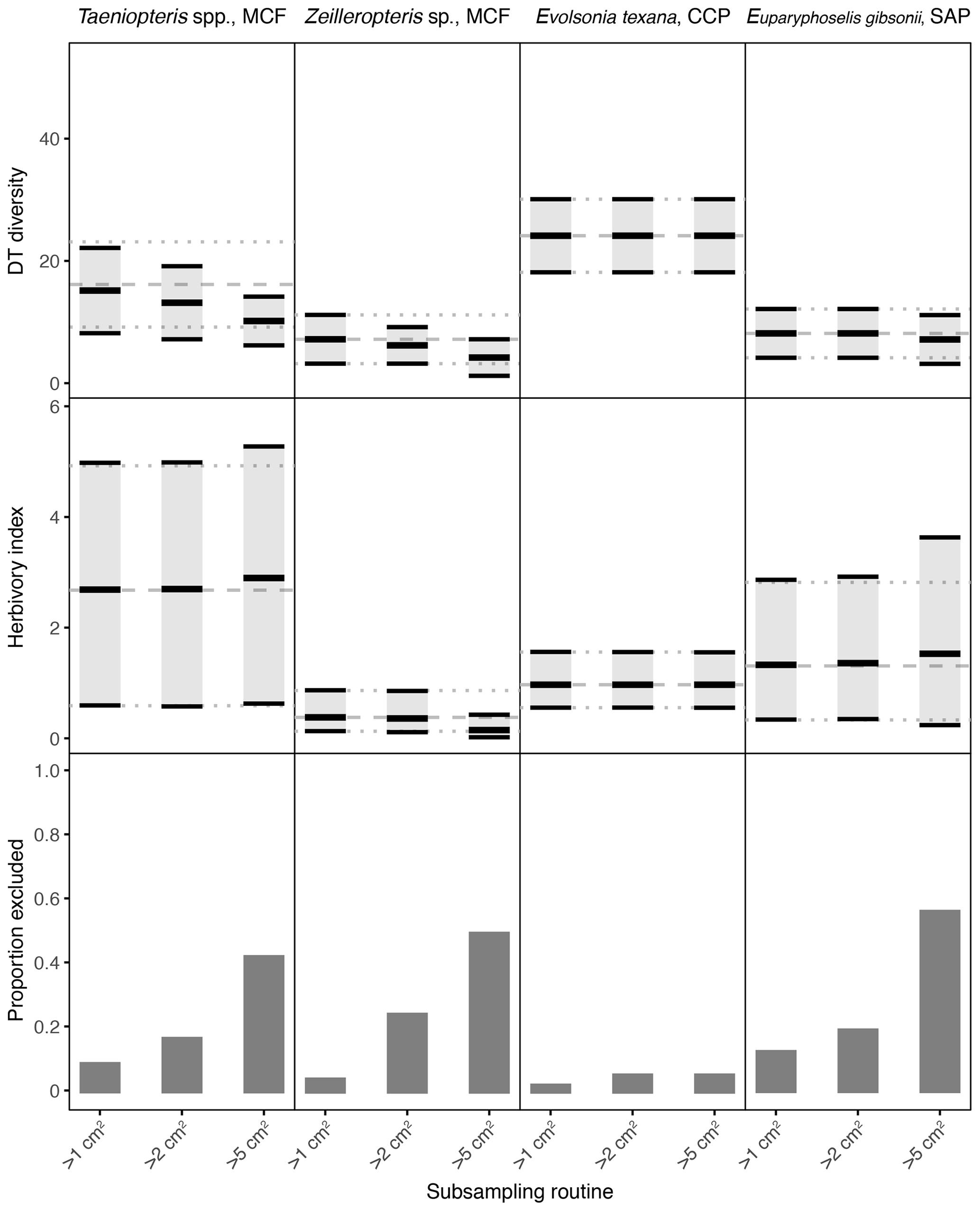
Figure 4Damage type (DT) diversity, the herbivory index (percentage of leaf area removed), and the proportion of specimens excluded, calculated with different specimen area restrictions, for the four primarily and secondarily dominant Permian plant hosts represented by fewer than 400 specimens. The dashed gray line represents the mean value calculated for the complete dataset, and the dotted gray lines represent the 95 % confidence intervals for the complete dataset. For the complete datasets, all specimens with a surface area above 0.5 cm2 were examined. The 95 % confidence interval for each subsampling routine is represented by a light gray rectangle bounded by black lines. The thick black lines represent the mean values for each subsampling routine.
Among the plant hosts represented by far fewer than 400 specimens, some resulting patterns are also clear from the complete datasets (Fig. 4). Evolsonia texana at CCP has higher DT diversity than Zeilleropteris sp. at MCF and Euparyphoselis gibsonii at SAP. Taeniopteris spp. at MCF yields a confidence interval for DT diversity that overlaps with those of all three secondarily dominant, gigantopterid plant hosts. The herbivory indices of all four of these plant hosts overlap. Taeniopteris spp. at MCF yields the widest confidence interval, and Zeilleropteris sp. and Evolsonia texana yield the narrowest confidence intervals.
3.2 Random sampling
When only a subset of the specimens are sampled, random sampling causes the confidence intervals to widen the most. When only 100 specimens are sampled randomly, the width of the confidence intervals often doubles (Fig. 2). When 200 specimens are sampled randomly, the confidence intervals narrow but are still noticeably wider than for the complete dataset. At both 100 and 200 randomly sampled specimens, the confidence interval for Johniphyllum multinerve at SAP overlaps with the confidence intervals for Auritifolia waggoneri and Taeniopteris spp. at CCP, although this overlap is not observed when the complete datasets are sampled (Fig. 2).
3.3 Sampling the largest specimens
When only the largest 100 specimens are sampled, confidence intervals can widen and mean values of DT diversity and the herbivory index can differ from the means calculated with the complete dataset. For Auritifolia waggoneri, the mean values of DT diversity and the herbivory index are minimally offset, but the width of the confidence intervals is noticeably larger than the width of the confidence intervals calculated with the complete dataset (Fig. 2). For Taeniopteris spp. at CCP, the mean value for DT diversity decreases noticeably when only the 100 largest specimens are sampled, and the mean value for the herbivory index increases slightly; the width of confidence intervals under this subsampling routine is very similar to the width of the confidence intervals calculated with the complete dataset (Fig. 2). For Johniphyllum multinerve at SAP, the mean value for DT diversity decreases noticeably when only the 100 largest specimens are sampled, as is also the case for Taeniopteris spp. at CCP (Fig. 2). The mean value for the herbivory index becomes noticeably lower and the confidence interval widens. When the 100 largest specimens are sampled, the confidence interval for DT diversity of J. multinerve at SAP does not overlap with the confidence intervals for A. waggoneri and Taeniopteris spp. of CCP. The confidence intervals for the herbivory index of Taeniopteris spp. and A. waggoneri at CCP do not overlap under this subsampling routine, but the confidence interval for J. multinerve at SAP does overlap with the confidence interval for A. waggoneri at CCP.
When the largest 200 specimens are sampled rather than the largest 100, the mean values for DT diversity and the herbivory index differ less from the true means and the confidence intervals narrow. For Auritifolia waggoneri at CCP, sampling of the largest 200 specimens yields mean values and confidence intervals that are nearly indistinguishable from those calculated from the complete dataset (Fig. 2). For Taeniopteris spp. at CCP, the mean value for DT diversity is noticeably lower than that calculated from the complete dataset, but the width of the confidence interval is nearly identical, and the mean value and confidence interval for the herbivory index are indistinguishable from those calculated from the complete dataset (Fig. 2). For Johniphyllum multinerve at SAP, the mean values for DT diversity and the herbivory index remain offset from the means calculated from the complete dataset, but the offset is slight compared to that seen when only the 100 largest specimens are sampled; the confidence interval for the herbivory index remains relatively wide (Fig. 2).
When 200 of the 250 largest specimens are sampled, the means and confidence intervals resemble those calculated from the 200 largest specimens. For Auritifolia waggoneri and Taeniopteris spp. at CCP, these two subsampling routines yield identical means and very similar confidence intervals (Fig. 2). For Johniphyllum multinerve at SAP, the mean values are less offset when 200 of the 250 largest specimens are sampled; the confidence interval for DT diversity widens slightly and the confidence interval for the herbivory index is minimally offset (Fig. 2). When the 200 largest specimens are sampled, or when 200 of the 250 largest specimens are sampled, patterns of overlap between different plant hosts' confidence intervals are identical to those recovered when the complete dataset is used for all calculations – though the distance between different plant hosts' confidence intervals is often reduced.
3.4 Increasing the minimum specimen size
When the threshold for minimum specimen area is increased from 0.5 to 1 cm2, the impact on mean values and confidence intervals is either negligible or indiscernible for all seven plant hosts examined here (Figs. 3, 4). When the threshold is increased to 2 cm2, the effect is again negligible for Auritifolia waggoneri and Taeniopteris spp. at CCP (Fig. 3). For the herbivory index for Johniphyllum multinerve at SAP, the lower bound of the 95 % confidence interval is nearly unchanged, the mean value increases slightly, and the upper bound of the 95 % confidence interval increases noticeably – although this widened confidence interval still does not overlap with that of A. waggoneri at CCP (Fig. 3). For Evolsonia texana at CCP and Euparyphoselis gibsonii at SAP, the increased sampling threshold of 2 cm2 does not have a meaningful impact on mean values or confidence intervals (Fig. 4). However, for the two plant hosts at MCF – Taeniopteris spp. and Zeilleropteris sp. – the 2 cm2 threshold causes a decrease in the mean values and confidence intervals for DT diversity, though the herbivory index is unaffected (Fig. 4).
When the threshold for minimum specimen area is then increased from 2 to 5 cm2, effects become more noticeable. The mean values and confidence intervals for Auritifolia waggoneri at CCP continue to resemble the values calculated from the complete dataset (Fig. 3). The same is true for the herbivory index of Taeniopteris spp. at CCP, but the mean value and confidence interval for DT diversity are noticeably offset below the values calculated from the complete dataset (Fig. 3). For Johniphyllum multinerve at SAP, DT diversity is offset below the true mean, far more so than is the case for Taeniopteris at CCP (Fig. 3). The mean value for the herbivory index is offset above the value calculated from the complete dataset, and the confidence interval is nearly twice the width of the confidence interval calculated from the complete dataset. This causes overlap of the confidence intervals calculated for the herbivory indices of A. waggoneri at CCP and J. multinerve at SAP, a result that is not recovered from the complete datasets.
For the plant hosts represented by fewer than 400 specimens, the changes caused by a 5 cm2 sampling threshold can be even more extreme. Results for Evolsonia texana at CCP are unaffected by this change in sampling threshold (Fig. 4); this is the only plant host for which only two specimens have a surface area below 5 cm2. For Euparyphoselis gibsonii at SAP, the 5 cm2 sampling threshold has a negligible impact on DT diversity. This threshold causes the mean value for the herbivory index to be slightly offset from the true mean and causes the confidence interval for the herbivory index to widen noticeably (Fig. 4). For Zeilleropteris sp. at MCF, the 95 % confidence intervals for both DT diversity and the herbivory index barely overlap with the true mean values when the sampling threshold is increased to 5 cm2 (Fig. 4). For Taeniopteris spp. at MCF, the 5 cm2 sampling threshold causes a slight change in values of the herbivory index and causes the entire 95 % confidence interval for DT diversity to fall well below the true mean (Fig. 4).
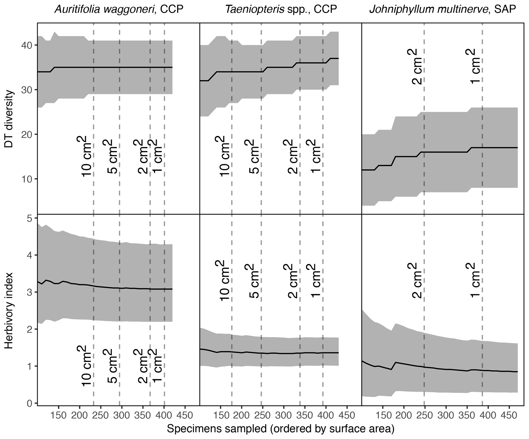
Figure 5Sequential increases in sample size, starting with the largest specimens, for the three primarily dominant Permian plant hosts represented by 400 or more specimens.
3.5 Sequential increases in sampling
When sampling increases sequentially, beginning with the 100 largest specimens and increasing with the next 10 largest until all specimens have been sampled, trends vary among plant hosts. For Auritifolia waggoneri at CCP, the mean value and confidence interval for DT diversity remain unchanged after the 220 largest specimens – measuring 11.36 cm2 and above – are sampled (Fig. 5). After the 200 largest specimens have been sampled, the mean value for the herbivory index decreases slightly and the upper bound of the confidence interval decreases more noticeably while the lower bound of the confidence interval remains virtually unchanged.
For Taeniopteris spp. at CCP and Johniphyllum multinerve at SAP, DT diversity shows a stepwise increase that continues well after the largest specimens have been sampled. For Taeniopteris spp., the confidence interval for DT diversity narrows as sampling increases, whereas the width of this confidence interval remains almost unchanged for J. multinerve at SAP (Fig. 5). As sampling increases, the herbivory index for Taeniopteris spp. at CCP decreases slightly and the confidence interval narrows noticeably. For J. multinerve at SAP these values change more dramatically, with the mean herbivory index decreasing, increasing, and decreasing again as sampling continues, while the confidence interval becomes far narrower (Fig. 5).
3.6 Nonmetric multidimensional scaling
3.6.1 Prediction ellipses
The prediction ellipses become smaller, and less likely to overlap, as sampling increases. Increased total sampling also decreases the size of prediction intervals for plant hosts, regardless of how much surface area is subsampled: the plant hosts that are represented by the highest amount of total surface area (Taeniopteris spp. and Auritifolia waggoneri at CCP) typically yield smaller prediction intervals than the plant hosts represented by less surface area.
There are no consistent patterns as to how the sizes of prediction ellipses change according to the dataset used. When all leaf specimens with a surface area above 0.5 cm2 are included in NMDS analyses, precision does not vary in a consistent manner between the presence–absence dataset and the surface-area datasets. For example, the prediction ellipse for CCP ceases to overlap with those for MCF and SAP once sampling increases from a total of 250 to 500 cm2 of surface area for both the presence–absence dataset (Figs. S5, S6 in the Supplement) and the surface-area datasets (Figs. S23, S24, S32, S33). This is not the case for the “cutoff” dataset in which Johniphyllum multinerve specimens with a surface area below 1.306 cm2 and Auritifolia waggoneri specimens with a surface area below 3.7 cm2 were excluded (Figs. S14, S15) – instead, with this dataset, the prediction ellipse for CCP only ceases to overlap with that for MCF once 1250 cm2 of leaf area has been sampled.
However, when individual plant hosts – instead of entire assemblages – are analyzed with NMDS, there is no discrepancy between the cutoff dataset and the presence–absence dataset that includes all specimens above 0.5 cm2 in surface area. The same pattern holds for both of these datasets: prediction ellipses for the two plant hosts from CCP cease to overlap with any other ellipses once sampling increases to 1000 cm2 (Figs. S4, S13). When surface-area data are used instead of presence–absence data, these prediction intervals cease to overlap at much lower levels of subsampling: once 500 cm2 of leaf area have been sampled, prediction ellipses for the two plant hosts from CCP cease to overlap with any other ellipses (Figs. S20, S29).
3.6.2 Hypothesis testing
The vast majority of all p values recovered from the NMDS hypothesis testing (6∕324, or 98.15 %) are equal to zero. This holds for all comparisons encompassing over 250 cm2 of surface area, for all comparisons involving CCP and its plant hosts, and for all comparisons with presence–absence data. Even the p values that are above zero are well below the significance threshold of 0.05. The tests that yielded p values above zero are as follows.
When assemblages were compared using 250 cm2 of surface area, with surface-area data, and with external foliage feeding groups kept separate, the majority of p values (5∕9) comparing MCF to SAP were equal to zero, with the remaining values ranging from 0.001 to 0.023. When plant hosts were compared using 250 cm2 of surface area, with surface-area data, and with external foliage feeding groups kept separate, one p value comparing Taeniopteris spp. from MCF to Johniphyllum multinerve from SAP was 0.002, with all other p values (8∕9) equal to zero. When assemblages were compared using 250 cm2 of surface area, with surface-area data, and with external foliage feeding groups lumped together, one p value comparing MCF to SAP was 0.012, with all other p values (8∕9) equal to zero.
4.1 Varying responses to subsampling among plant hosts
Plant hosts' responses to subsampling routines correspond to their morphological variability. Auritifolia waggoneri at CCP, a monophyletic plant host with low morphological variability, yields the most accurate results under the different subsampling routines examined here. When at least 200 specimens of A. waggoneri are examined, with preference given to the larger specimens, subsampling yields results that are similar to, or indistinguishable from, the results calculated from the complete dataset (Figs. 2, 3).
The dimorphic foliage of Johniphyllum multinerve at SAP can be split into two forms, here called Form 1 and Form 2. In addition to being more morphologically variable than A. waggoneri, J. multinerve is also more sensitive to subsampling routines. For example, sampling of the 100 largest specimens of A. waggoneri causes a very slight offset relative to the mean value calculated from the complete dataset; however, this same subsampling routine causes a far more dramatic offset of the mean value – and associated confidence intervals – for J. multinerve (Fig. 2). By contrast, Taeniopteris is the only plant category examined here that is known to be polyphyletic. At CCP, Taeniopteris spp. shows similarly high sensitivity to various subsampling routines (Figs. 2, 3). At MCF, where this plant host is represented by just slightly more than 100 specimens, subsampling can have an even more dramatic effect (Fig. 4).
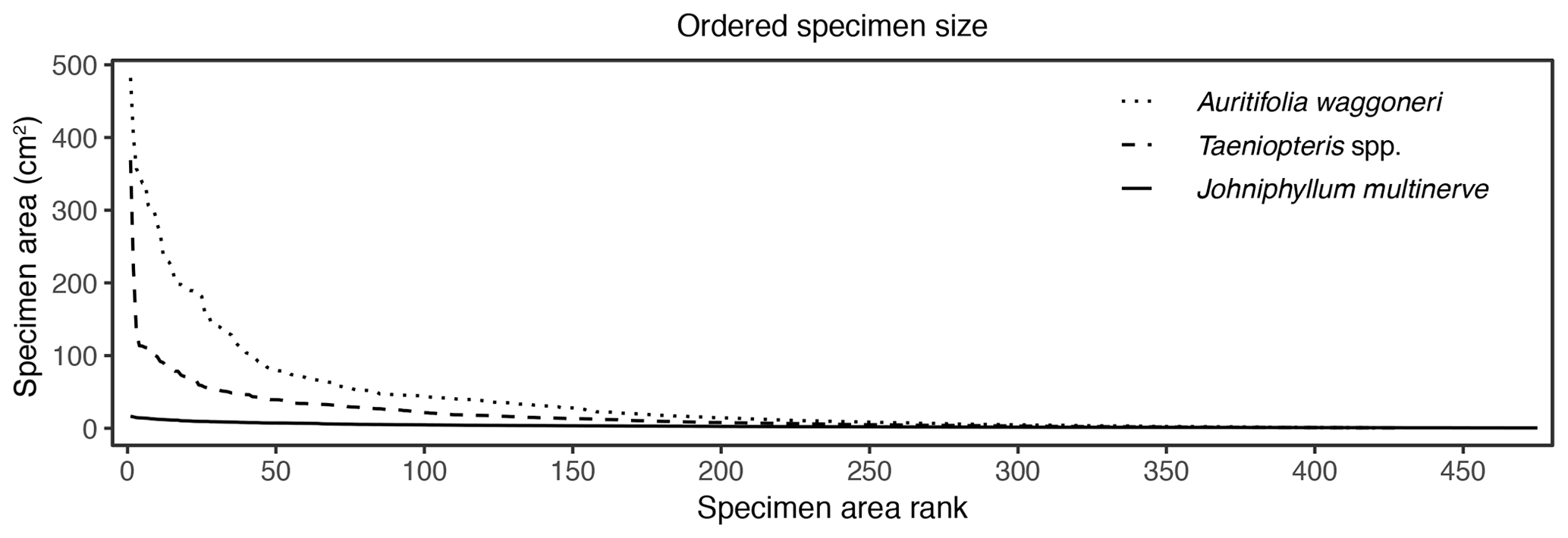
Figure 6Surface area of individual specimens, ordered by area for each plant host, for Auritifolia waggoneri and Taeniopteris spp. of CCP and Johniphyllum multinerve at SAP.
In addition to morphological variability, differences in the size of available leaf fragments may also play a role in sensitivity to subsampling routines. This almost certainly is the case for Johniphyllum multinerve at SAP, which is represented by relatively small fragments (Fig. 6). Of the 475 specimens representing J. multinerve, only 89, or 18.73 %, have a surface area greater than 5 cm2. It is probably for this reason that a minimum surface-area threshold of 5 cm2 causes noticeable changes in the estimated DT diversity and herbivory index for this taxon (Fig. 3). Furthermore, the two forms of J. multinerve differ in abundance, fragment size, and patterns of herbivory. Form 1 is represented by 112 specimens, which have an average surface area of 4.00 cm2; the three largest specimens belong to Form 1 (Fig. 7). Form 2 is represented by 363 specimens, which have an average surface area of 2.92 cm2. Because Form 1 is less common, large fragments belonging to Form 2 are approximately three times as abundant as large fragments belonging to Form 1 (Fig. 7). Form 1 also includes 14 out of 20, or 70 %, of the herbivorized J. multinerve specimens, despite its relative rarity (Fig. 8).
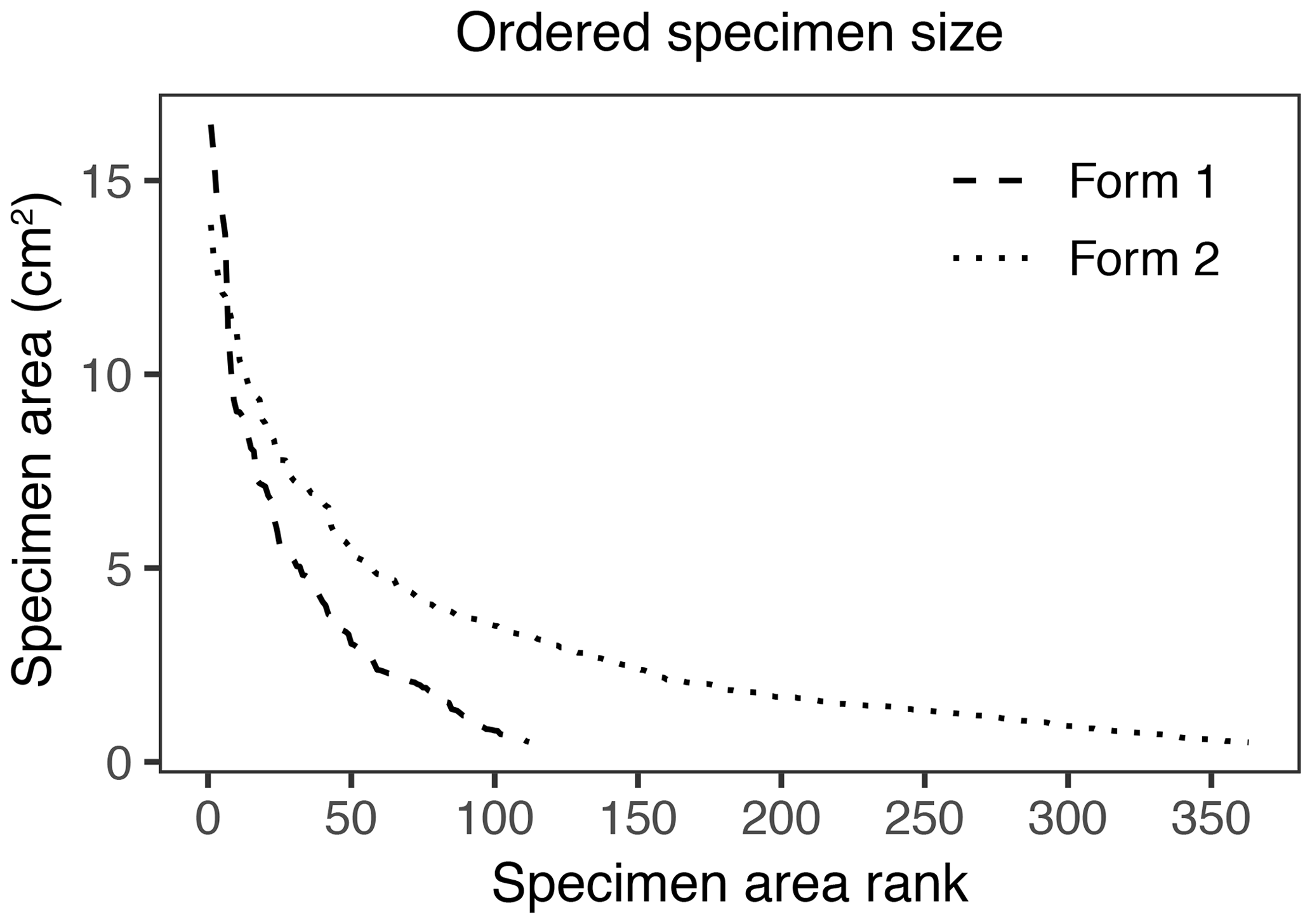
Figure 7Surface area of individual specimens ordered by area for the two forms of Johniphyllum multinerve at SAP.
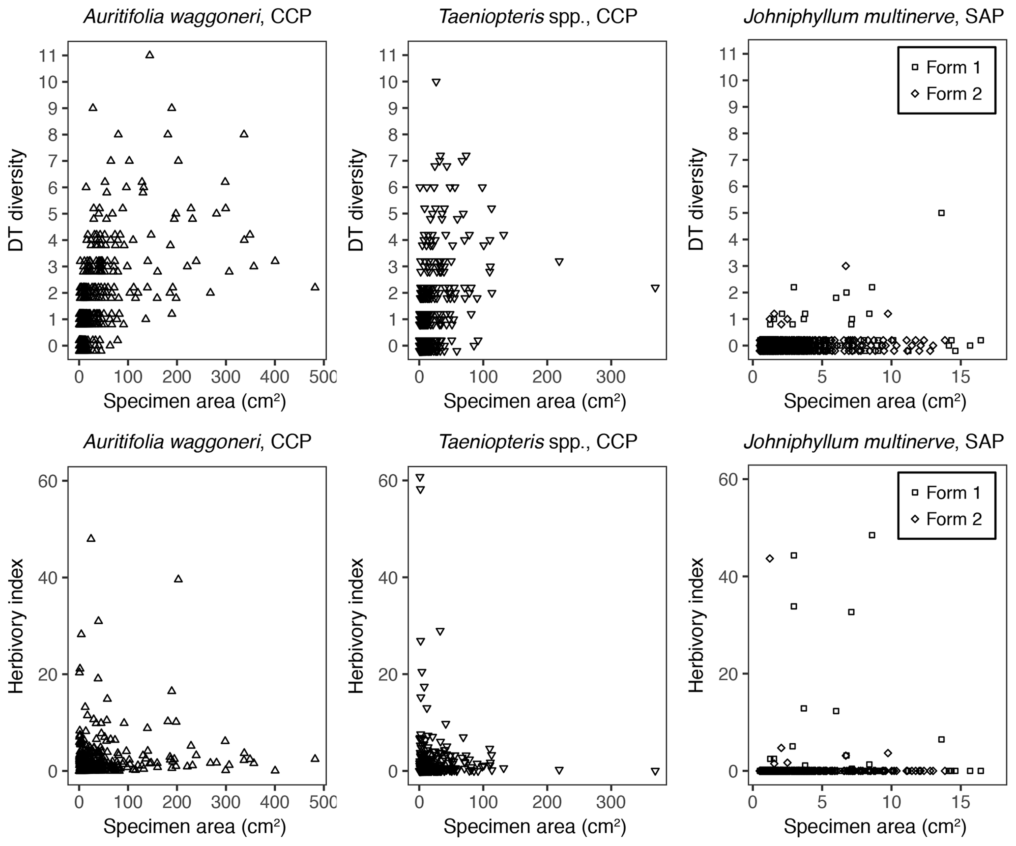
Figure 8The DT diversity and the herbivory index of each specimen, plotted against its surface area.
The size differences between the two primarily dominant plant hosts at CCP may also contribute to their differing responses to subsampling. These two plant hosts are represented by nearly identical numbers of specimens – 421 for Auritifolia waggoneri and 430 for Taeniopteris spp. – but differ in surface area. Of the largest 35 specimens that represent these two plant hosts, 33 belong to A. waggoneri. The 150 largest specimens of A. waggoneri are noticeably larger than the corresponding specimens belonging to Taeniopteris spp. (Fig. 6). At CCP, the 200 largest specimens of A. waggoneri have over twice as much total surface area as the 200 largest specimens of Taeniopteris spp. This may be one reason why the 200 largest specimens of A. waggoneri contain evidence for every DT found on this plant host at CCP, whereas the 200 largest specimens of Taeniopteris spp. lack the three DTs that are found on smaller specimens belonging to this same plant host (Moles and Westoby, 2000). The polyphyletic nature and varying host-plant specificities of the insect herbivores on Taeniopteris spp. at CCP may also be a reason why the 200 largest specimens do not contain evidence of all DTs. Some herbivores, and the DTs they produce, may be restricted to larger Taeniopteris specimens with cycadophyte affinities, and other herbivores producing a distinct suite of DTs may be restricted to smaller Taeniopteris specimens that appear to contain sporangia and are, therefore, interpreted to be ferns.
4.2 The utility of a priori subsampling thresholds
When the threshold for minimum specimen area is raised from 0.5 to 1 cm2, the effect on DT diversity and the herbivory index is minimal (Figs. 3, 4). This finding suggests that previous studies, which examined all fragments over 0.5 cm2 in surface area (Schachat et al., 2014, 2015; Maccracken and Labandeira, 2019), took an unnecessarily conservative approach and that future studies can safely exclude all fragments less than 1 cm2. Furthermore, storage space for paleobotanical collections is often an issue. If storage space for a Paleozoic flora is limited, the leaves under 1 cm2 may be photographed as voucher specimens and then discarded in the field.
When the threshold for minimum specimen area is raised to 2 cm2, the effects are more noticeable but do not increase the amount of overlap between confidence intervals (Figs. 3, 4). Therefore, for the plant hosts examined here, these effects are not strong enough to cause Type II errors. The most noticeable effects of the threshold increase from 1 to 2 cm2 can be seen in the DT diversity of Taeniopteris at MCF (Fig. 4), a polyphyletic fossil genus that is barely represented by 100 specimens despite being the dominant plant host in its assemblage. In terms of morphology, evolutionary history, and sample size, Taeniopteris spp. at MCF can be considered a paleobotanical worst-case example. Nevertheless, no Type II error results from the offset of the mean value and confidence interval for DT diversity for this taxon. This finding suggests that exclusion of all leaf fragments under 2 cm2 would be a defensible subsampling strategy for future studies. None of the other a priori subsampling criteria implemented here – a minimum surface area of 5 cm2, subsampling of a uniform number of random specimens, or subsampling of a uniform number of the largest specimens – yield consistently accurate results.
4.3 A sequential approach to subsampling
The sequential approach taken here suggests another, albeit slightly more complicated, way in which sampling effort can be minimized. In the sequential approach presented here, the 100 largest specimens are sampled, followed by the next largest specimens in groups of 10. Under this sequential subsampling approach, sampling can cease when both the mean value and confidence interval for DT diversity remain unchanged while the most recent 100 specimens have been sampled, assuming that the herbivory index also changes minimally.
When the 150 largest specimens had been sampled for Auritifolia waggoneri at CCP, the mean value for DT diversity reached 35 and the 95 % confidence interval ranged from 28 to 42 (Fig. 5). When sampling increased from the 150 largest specimens to the 250 largest specimens, these values remained unchanged and the relevant values for the herbivory index changed minimally. Under the sequential subsampling routine proposed here, sampling would cease at 250 specimens; at this level of sampling, results for DT diversity match those calculated from the complete dataset and results for the herbivory index are nearly indistinguishable from those calculated from the complete dataset. With this sequential approach, the smallest specimen sampled would be that which has a surface area of 8.41 cm2; the exclusion of all specimens measuring between 2 and 8.4 cm2 would represent a noticeable reduction in sampling effort without any meaningful effect on the results.
For Taeniopteris spp. at CCP, the mean value and confidence interval for DT diversity was not constant while 100 specimens are sampled sequentially by surface area (Fig. 5). Under the sequential subsampling routine, all specimens of Taeniopteris spp. at CCP would be sampled until the minimum size threshold of 1 or 2 cm2 is reached. The necessity of exhaustive sampling, of specimens of all size classes, is likely caused by the polyphyletic nature of this group.
When the 240 largest Johniphyllum multinerve specimens at SAP were sampled, the mean value for DT diversity reached 16 and the 95 % confidence interval ranged from 7 to 25 (Fig. 5). When sampling increased from the 240 to the 340 largest specimens, these values remained unchanged and the relevant values for the herbivory index changed minimally. At this level of sampling, values for DT diversity are only offset slightly (by one DT) from the values calculated from the complete dataset, and values for the herbivory index are essentially indistinguishable from those calculated from the complete dataset. With this sequential approach, the smallest specimen sampled would be that which has a surface area of 1.306 cm2 – sampling would have continued past the minimum size threshold of 2 cm2. However, if sampling had stopped when the minimum size threshold of 2 cm2 was reached, the results for DT diversity would be exactly the same and the confidence interval for the herbivory index would only be slightly wider. This finding suggests that a minimum size threshold and sequential sampling are compatible. Accordingly, specimens can be sampled sequentially from largest to smallest, continuing either until the addition of 100 specimens has not changed the results for DT diversity or until the minimum size threshold has been reached.
Unlike Auritifolia waggoneri and Taeniopteris spp., Johniphyllum multinerve at SAP can be divided into two separate forms, simply called Form 1 and Form 2 here. Form 1 is represented by only 112 specimens and, therefore, is not amenable to the sequential subsampling routine suggested here. However, for more abundant plant hosts that are represented by multiple, discrete forms, the sequential subsampling routine proposed here could be implemented separately for each form, with results presented individually for each form and in combination for the plant host as a whole. This approach would have two advantages. First, sequentially sampled data would not be confounded by differences in DT composition and specimen size between forms, such that results may stabilize earlier. Second, the collection of a separate dataset for each form of each plant host would facilitate more nuanced interpretations of insect herbivory: for example, if the two forms of a plant host correspond to sun leaves and shade leaves, these forms may host different component communities of insect herbivores.
4.4 The impact of subsampling on NMDS results
Because prediction ellipses are generally smaller when calculated from the surface-area datasets than when calculated from the presence–absence datasets, we recommend using surface-area data for NMDS. Because prediction ellipses become noticeably smaller when sampling increases from 1000 to 750 cm2, we recommend sampling at least 1000 cm2 of leaf area for plant hosts and assemblages included in NMDS plots created with surface-area data. Because prediction ellipses continue to shrink noticeably at 1250 cm2 of surface area when presence–absence data are used, we recommend sampling at least 1500 cm2 of leaf area for plant hosts and assemblages included in NMDS plots created with presence–absence data. When prediction ellipses are generated in increasing intervals of 250 cm2 of surface area, sampling can be considered sufficient once the size of prediction intervals ceases to decrease. Because the plant hosts represented by the highest total surface area (Auritifolia waggoneri and Taeniopteris spp. from CCP) yield noticeably smaller prediction ellipses at all levels of sampling, we are not able to designate a surface-area threshold at which sampling can be considered exhaustive in the context of NMDS.
The exclusion of smaller specimens has a noticeable impact on the presence–absence dataset for Auritifolia waggoneri but not for Johniphyllum multinerve. When we excluded the 321st-largest through smallest specimen of A. waggoneri, because DT diversity did not change after we sampled the 220th-largest specimen from this species, NMDS confidence intervals for A. waggoneri became more likely to overlap with those of Taeniopteris spp. at MCF. The exclusion of the smallest specimens, therefore, made it more difficult to distinguish herbivore communities that appear to be distinct when visualized with complete datasets, even though the mean and confidence interval for DT diversity remained stable.
As evaluated with NMDS, CCP and MCF have herbivore communities that are so different that not only are all relevant p values equal to zero but their prediction intervals do not overlap. However, the herbivore communities for these two assemblages were originally described as being very similar, and at first glance appeared to be so (Schachat et al., 2014, 2015). This finding raises the possibility that nearly all herbivore communities in the fossil record will appear significantly different when a minimum amount of leaf area is sampled, in which case p values of zero cannot be interpreted as reflecting any particular biological phenomenon, such as evolution or response to climate change. When NMDS is used to evaluate multiple assemblages belonging to different categories, such as studies in which various geologic intervals are each represented by multiple assemblages (Wappler et al., 2009; Currano et al., 2010), pairwise distances between centroids can be compared within and between intervals.
4.5 Future directions
The minimum fragment threshold and the sequential subsampling routine suggested here should be validated with studies of additional plant hosts, particularly angiosperms and needle-leaved conifers. One issue with the plant hosts examined here is that the vast majority of specimens are, in fact, fragments; the size of each specimen is partly a function of leaf area, in that a specimen cannot be larger than the leaf from which it came, but is largely a function of fragmentation. Sampling routines that proceed sequentially from the largest to the smallest specimens prioritize the most complete specimens to a greater extent than they prioritize the largest leaves. And for the plant hosts examined here, it is often impossible to estimate whether a given fragment represents 50 % or more of the original leaf area – for example, many Taeniopteris fragments are missing both the base and the apex of the leaf, and the width of a leaf is insufficient to estimate its length due to the variable morphology and size of this polyphyletic group.
Sampling of angiosperms often differs from sampling of the gymnospermous plant hosts examined here in that the only specimens sampled are typically those that include at least 50 % of the inferred original leaf area. For such plant hosts, sequential sampling of the largest to smallest specimens may not be necessary. A random subsampling approach would be more likely to work with angiosperms, and sampling could continue until the addition of 100 leaves does not change the results for DT diversity as outlined above. However, due to high similarity between the vein architecture of many angiosperms within a flora – as well as the significantly greater leaf diversity in a typical angiosperm flora compared to a gymnosperm flora – only strictly identifiable angiosperm fragments should be used: those assignable to a Linnaean species or to a defined morphotype. Consequently, the minimum size of the fragments would likely be greater than those of gymnosperms. Future studies could examine the extent to which random sampling, rather than sequential sampling by specimen area, works for plant hosts for which specimens are only sampled when at least 50 % complete.
Regardless of future results pertaining to the minimum fragment size threshold and the utility of a sequential sampling approach, data on insect herbivory in the fossil record will be of greater utility if measurements of herbivorized surface area are partitioned by damage type or at least by functional feeding group. Data collected in this manner would be conductive to nonmetric multidimensional scaling and would have the potential to reveal previously overlooked patterns in the evolution of insect herbivory.
The results presented here support the following preliminary guidelines for the sampling of fossil leaves in studies of insect herbivory.
-
For leaf fragments, a size threshold of either 1 or 2 cm2 should be used. A threshold of 2 cm2 appears to have little effect on the final results for plant hosts that are monophyletic, whereas a more conservative threshold of 1 cm2 may be necessary for polyphyletic groups such as Taeniopteris from the Permian of Texas.
-
For plant hosts represented by over 200 specimens, a sequential approach can be taken for sampling. Specimens are sampled sequentially from largest to smallest, or from most to least complete, and sampling ends either when the minimum size threshold has been reached (see the first item in this list) or when the addition of 100 specimens to the dataset has had no effect on DT diversity and a minimum effect of the herbivory index.
-
For plant hosts that include multiple discrete morphological forms, for which each form is represented by over 200 specimens, this sequential approach can be taken for each form rather than for the plant host as a whole.
-
At least 1000 cm2 of surface area should be examined for all plant hosts and assemblages included in NMDS plots created with surface-area data, and at least 1500 cm2 of surface area should be examined for all plant hosts and assemblages included in NMDS plots created with presence–absence data.
-
To evaluate whether sampling is sufficient for NMDS, 84 % prediction ellipses should be generated from subsampled data in NMDS plots at levels of subsampling that iteratively increase by 250 cm2.
-
To evaluate differences in insect herbivory in the context of NMDS, p values should be generated by testing the hypothesis that the distances between centroids are equal to the distances seen when the same assemblage/plant host is subsampled twice.
-
For studies in which each geologic interval is represented by multiple assemblages, the mean pairwise distances between assemblages' centroids should be reported from NMDS plots, within and between intervals.
All data, results, and code are available at https://purl.stanford.edu/vk558vn8658 (last access: 11 February 2020) (Schachat et al., 2019) under a CC BY-NC Attribution-NonCommercial license.
All data used here were collected from specimens housed in the Paleobiology Collections of the Smithsonian Institution. Herbivory on these specimens has been described by Schachat et al. (2014), Schachat et al. (2015), and Maccracken and Labandeira (2019).
The supplement related to this article is available online at: https://doi.org/10.5194/fr-23-15-2020-supplement.
SRS conceived the study, analyzed data, and drafted the initial version of the manuscript. SRS, CCL, and SAM contributed to writing and editing the manuscript.
The authors declare that they have no conflict of interest.
We thank Steve Wang for help with methods development and with computing. We thank two anonymous reviewers for thoughtful and constructive feedback on this paper. We thank William A. DiMichele, Dan S. Chaney, and Cindy Looy for help with identification and description of the plant hosts at MCF, CCP, and SAP. We thank Alan Rulis for measuring specimen surface area from SAP. This is contribution 371 to the Evolution of Terrestrial Ecosystems consortium at the National Museum of Natural History, in Washington, D.C.
Sandra R. Schachat was funded by the Chair's Fellowship of the Stanford University Department of Geological Sciences and is funded as a Coleman F. Fung Interdisciplinary Graduate Fellow through the Stanford Interdisciplinary Graduate Fellowship program. S. Augusta Maccracken is funded by the Big Ten Academic Alliance Smithsonian Predoctoral Fellowship.
This paper was edited by Torsten Scheyer and reviewed by two anonymous referees.
Beck, A. L. and Labandeira, C. C.: Early Permian Insect Folivory on a Gigantopterid-Dominated Riparian Flora from North-Central Texas, Palaeogeogr. Palaeocl., 142, 139–173, 1998. a
Béthoux, O., Galtier, J., and Nel, A.: Earliest Evidence of Insect Endophytic Oviposition, Palaios, 19, 408–413, https://doi.org/10.1669/0883-1351(2004)019<0408:EEOIEO>2.0.CO;2, 2004. a
Bowen, Z. and Freeman, M.: Sampling Effort and Estimates of Species Richness Based on Prepositioned Area Electrofisher Samples, N. Am. J. Fish. Manage., 18, 144–153, 1998. a
Brenner, G. J.: Evidence for the Earliest Stage of Angiosperm Pollen Evolution: A Paleoequatorial Section from Israel, in: Flowering Plant Origin, Evolution & Phylogeny, pp. 91–115, Springer, New York, 1996. a
Chaney, D. S., Sues, H.-D., and DiMichele, W. A.: A Juvenile Skeleton of the Nectridean Amphibian Diplocaulus and Associated Flora and Fauna from the Mitchell Creek Flats Locality (Upper Waggoner Ranch Formation; Early Permian), Baylor County, North-Central Texas, USA, New Mexico Museum of Natural History and Science Bulletin, Albuquerque, New Mexico, pp. 39–47, 2005. a
Chaney, D. S., Mamay, S. H., DiMichele, W. A., and Kerp, H.: Auritifolia Gen. Nov., Probable Seed Plant Foliage with Comioid Affinities from the Early Permian of Texas, U.S.A., Int. J. Plant Sci., 170, 247–266, https://doi.org/10.1086/595293, 2009. a
Currano, E. D., Labandeira, C. C., and Wilf, P.: Fossil Insect Folivory Tracks Paleotemperature for Six Million Years, Ecol. Monogr., 80, 547–567, https://doi.org/10.1890/09-2138.1, 2010. a, b, c, d
Currano, E. D., Jacobs, B. F., Pan, A. D., and Tabor, N. J.: Inferring Ecological Disturbance in the Fossil Record: A Case Study from the Late Oligocene of Ethiopia, Palaeogeogr. Palaeocl., 309, 242–252, https://doi.org/10.1016/j.palaeo.2011.06.007, 2011. a
Ding, Q., Labandeira, C. C., Meng, Q., and Ren, D.: Insect Herbivory, Plant-Host Specialization and Tissue Partitioning on Mid-Mesozoic Broadleaved Conifers of Northeastern China, Palaeogeogr. Palaeocl., 440, 259–273, https://doi.org/10.1016/j.palaeo.2015.09.007, 2015. a
Droissert, V., Hardy, O., Sonke, B., Dahdouh-Guebas, F., and Stevart, T.: Subsampling Herbarium Collections to Assess Geographic Diversity Gradients: A Case Study with Endemic Orchidaceae and Rubiaceae in Cameroon, Biotropica, 44, 44–52, 2012. a
England, J. R. and Attiwill, P. M.: Changes in Leaf Morphology and Anatomy with Tree Age and Height in the Broadleaved Evergreen Species, Eucalyptus regnans F. Muell, Trees, 20, 79–90, 2006. a
Filho, E. B. D. S., Adami-Rodrigues, K., de Lima, F. J., Bantim, R. A. M., Wappler, T., and Saraiva, A. Á. F.: Evidence of Plant–Insect Interaction in the Early Cretaceous Flora from the Crato Formation, Araripe Basin, Northeast Brazil, Hist. Biol., 31, 926–937, https://doi.org/10.1080/08912963.2017.1408611, 2019. a
Gifford, E. M. E. M. and Foster, A. S.: Morphology and Evolution of Vascular Plants, Tech. rep., W.H. Freeman and Company, New York, 1989. a
Glasspool, I., Hilton, J., Collinson, M., and Wang, S. J.: Foliar Herbivory in Late Palaeozoic Cathaysian Gigantopterids, Rev. Palaeobot. Palyno., 127, 125–132, https://doi.org/10.1016/S0034-6667(03)00107-6, 2003. a
Gotelli, N. and Colwell, R.: Chapter 4: Estimating Species Richness, in: Biological Diversity, Frontiers in Measurement and Assessment, edited by: Magurran, A. and McGill, B., 2, 39–54, https://doi.org/10.2307/3547060, 2011. a
Iannuzzi, R. and Labandeira, C. C.: The Oldest Record of External Foliage Feeding and the Expansion of Insect Folivory on Land, Ann. Entomol. Soc. Am., 101, 79–94, https://doi.org/10.1603/0013-8746(2008)101[79:TOROEF]2.0.CO;2, 2008. a
Jud, N. A. and Sohn, J. C.: Evidence for an Ancient Association between Leaf Mining Flies and Herbaceous Eudicot Angiosperms, Cretaceous Res., 63, 113–121, https://doi.org/10.1016/j.cretres.2016.02.019, 2016. a
Karban, R. and Baldwin, I. T.: Induced Responses to Herbivory, University of Chicago Press, Chicago and London., 2007. a
Knor, S., Skuhravá, M., Wappler, T., and Prokop, J.: Galls and Gall Makers on Plant Leaves from the Lower Miocene (Burdigalian) of the Czech Republic: Systematic and Palaeoecological Implications, Rev. Palaeobot. Palyno., 188, 38–51, https://doi.org/10.1016/j.revpalbo.2012.10.001, 2013. a
Kodrul, T. M., Maslova, N. P., Vasilenko, D. V., Herman, A. B., Xu, Q., Jin, J., and Liu, X.: A Preliminary Assessment of Plant–Biotic Interactions in the Eocene of South China: Evidence from Liquidambar L. (Saxifragales: Altingiaceae), Palaeogeogr. Palaeocl., 492, 147–160, https://doi.org/10.1016/j.palaeo.2017.12.020, 2018. a
Kruskal, J. B. and Wish, M.: Multidimensional Scaling. Number 07–011 in Sage University Paper Series on Quantitative Applications in the Social Sciences, Newberry Park, California, 1978. a
Labandeira, C. C.: Insect Mouthparts: Ascertaining the Paleobiology of Insect Feeding Strategies, Annu. Rev. Ecol. Syst., 28, 153–193, https://doi.org/10.1146/annurev.ecolsys.28.1.153, 1997. a
Labandeira, C. C. and Allen, E. G.: Minimal Insect Herbivory for the Lower Permian Coprolite Bone Bed Site of North-Central Texas, USA, and Comparison to Other Late Paleozoic Floras, Palaeogeogr. Palaeocl., 247, 197–219, https://doi.org/10.1016/j.palaeo.2006.10.015, 2007. a
Labandeira, C. C., Wilf, P., Johnson, K. R., and Marsh, F.: Guide to Insect (and Other) Damage Types on Compressed Plant Fossils (Version 3.0), Smithsonian Institution, Washington D.C., 2007. a
Labandeira, C. C., Tremblay, S. L., Bartowski, K. E., and VanAller Hernick, L.: Middle Devonian Liverwort Herbivory and Antiherbivore Defence, New Phytologist, 200, 247–258, https://doi.org/10.1111/nph.12643, 2013. a
Labandeira, C. C., Anderson, J. M., and Anderson, H. M.: Expansion of Arthropod Herbivory in Late Triassic South Africa: The Molteno Biota, Aasvoëlberg 411 Site and Developmental Biology of a Gall, in: The Late Triassic World: Earth in a Time of Transition, edited by: Tanner, L. H., pp. 623–719, Springer International Publishing, Cham, https://doi.org/10.1007/978-3-319-68009-5_14, 2018. a
Looy, C. V. and Duijnstee, I.: Voltzian Conifers of the South Ash Pasture Flora (Guadalupian, Texas): Johniphyllum multinerve Gen. et Sp. Nov., Pseudovoltzia sapflorensis Sp. Nov., and Wantus acaulis Sp. Nov., Int. J. Plant Sci., published online, https://doi.org/10.1086/706853, 2019. a, b
Maccracken, S. and Labandeira, C. C.: The Middle Permian South Ash Pasture Assemblage of North-Central Texas: Coniferophyte and Gigantopterid Herbivory and Longer-Term Herbivory Trends, Int. J. Plant Sci., published online, https://doi.org/10.1086/706852, 2019. a, b, c
McLoughlin, S., Martin, S. K., and Beattie, R.: The Record of Australian Jurassic Plant–Arthropod Interactions, Gondw. Res., 27, 940–959, https://doi.org/10.1016/j.gr.2013.11.009, 2015. a
Meng, Q.-M., Labandeira, C. C., Ding, Q.-L., and Ren, D.: The Natural History of Oviposition on a Ginkgophyte Fruit from the Middle Jurassic of Northeastern China, Insect Sci., 26, 171–179, https://doi.org/10.1111/1744-7917.12506, 2017. a
Moles, A. and Westoby, M.: Do Small Leaves Expand Faster than Large Leaves, and Do Shorter Expansion Times Reduce Herbivore Damage?, Oikos, 90, 517–524, 2000. a
Oksanen, J., Blanchet, F. G., Friendly, M., Kindt, R., Legendre, P., McGlinn, D., Minchin, P. R., O'Hara, R., Simpson, G. L., Solymos, P., Stevens, M. H. H., Szoecs, E., and Wagner, H.: vegan: Community Ecology Package, R Package Version 2.4-4, 2018. a
Pilliod, D. and Arkle, R.: Performance of Quantitative Vegetation Sampling Methods across Gradients of Cover in Great Basin Plant Communities, Rangeland Ecol. Manag., 66, 634–647, 2013. a
Pinheiro, E. R. S., Iannuzzi, R., and Duarte, L. D. S.: Insect Herbivory Fluctuations through Geological Time, Ecology, 97, 2501–2510, https://doi.org/10.1002/ecy.1476, 2016. a, b, c, d
Pires, E. F. and Sommer, M. G.: Plant-Arthropod Interaction in the Early Cretaceous (Berriasian) of the Araripe Basin, Brazil, J. S. Am. Earth Sci., 27, 50–59, https://doi.org/10.1016/j.jsames.2008.09.004, 2009. a
R Development Core Team: R: A Language and Environment for Statistical Computing, R Foundation for Statistical Computing, Vienna, Austria, 2017. a
Sarijeva, G., Knapp, M., and Lichtenthaler, H.: Differences in Photosynthetic Activity, Chlorophyll and Carotenoid Levels, and in Chlorophyll Fluorescence Parameters in Green Sun and Shade Leaves of Ginkgo and Fagus, J. Plant Physiol., 164, 950–955, 2007. a
Schachat, S. R., Labandeira, C. C., Gordon, J., Chaney, D., Levi, S., Halthore, M. N., and Alvarez, J.: Plant–Insect Interactions from Early Permian (Kungurian) Colwell Creek Pond, North-Central Texas: The Early Spread of Herbivory in Riparian Environments, Int. J. Plant Sci., 175, 855–890, https://doi.org/10.1086/677679, 2014. a, b, c, d, e, f
Schachat, S. R., Labandeira, C. C., and Chaney, D. S.: Insect Herbivory from Early Permian Mitchell Creek Flats of North-Central Texas: Opportunism in a Balanced Component Community, Palaeogeogr. Palaeocl., 440, 830–847, https://doi.org/10.1016/j.palaeo.2015.10.001, 2015. a, b, c, d, e
Schachat, S. R., Labandeira, C. C., and Maccracken, S. A.: The Importance of Sampling Standardization for Comparisons of Insect Herbivory in Deep Time: A Case Study from the Late Palaeozoic, Roy. Soc. Open Sci., 5, 171991, https://doi.org/10.1098/rsos.171991, 2018. a, b
Schachat, S. R., Maccracken, S. A., and Labandeira, C. C.: Data and code from “Sampling fossil floras for the study of insect herbivory: how many leaves is enough?”, Stanford Digital Repository, available at: https://purl.stanford.edu/vk558vn8658 (last access: 11 February 2020), 2019. a
Slater, B. J., McLoughlin, S., and Hilton, J.: Animal–Plant Interactions in a Middle Permian Permineralised Peat of the Bainmedart Coal Measures, Prince Charles Mountains, Antarctica, Palaeogeogr. Palaeocl., 363–364, 109–126, https://doi.org/10.1016/j.palaeo.2012.08.018, 2012. a
Smith, D. M.: A Comparison of Plant–Insect Associations in the Middle Eocene Green River Formation and the Upper Eocene Florissant Formation and Their Climatic Implications, Geol. Soc. Am. Special Paper, 435, 89–103, https://doi.org/10.1130/2008.2435(06), 2008. a
Strullu-Derrien, C., McLoughlin, S., Philippe, M., Mørk, A., and Strullu, D. G.: Arthropod Interactions with Bennettitalean Roots in a Triassic Permineralized Peat from Hopen, Svalbard Archipelago (Arctic), Palaeogeogr. Palaeocl., 348–349, 45–58, https://doi.org/10.1016/j.palaeo.2012.06.006, 2012. a
Wappler, T. and Denk, T.: Herbivory in Early Tertiary Arctic Forests, Palaeogeogr. Palaeocl., 310, 283–295, https://doi.org/10.1016/j.palaeo.2011.07.020, 2011. a
Wappler, T., Currano, E. D., Wilf, P., Rust, J., and Labandeira, C. C.: No Post-Cretaceous Ecosystem Depression in European Forests? Rich Insect-Feeding Damage on Diverse Middle Palaeocene Plants, Menat, France, P. Roy. Soc. B-Biol. Sci., 276, 4271–4277, https://doi.org/10.1098/rspb.2009.1255, 2009. a, b
Wickham, H.: ggplot2: Elegant Graphics for Data Analysis, Springer, New York, 2009. a
Xu, Q., Jin, J., and Labandeira, C. C.: Williamson Drive: Herbivory on a North-Central Texas Flora of Latest Pennsylvanian Age Shows Discrete Component Community Structure, Expansion of Piercing and Sucking, and Plant Counterdefenses, Rev. Palaeobot. Palyno., 251, 28–72, https://doi.org/10.1016/j.revpalbo.2018.01.002, 2018. a, b
traceson leaves shows us how insects have adapted to changing climates. Here, we address the question of how many leaves from a single fossil locality must be examined to permit statistically robust comparisons in deep time.